Tutorial 2: Simple Mineral Prospectivity Maps with Kalpa

Tutorial by

Utpal Singh¹, Satyam Pratap Singh¹, Sourabh Motiani²

¹ School of Geosciences, University of Sydney

² Department of Earth Sciences, Indian Institute of Technology Roorkee

---

In this tutorial, we will use Kalpa to build a mineral prospectivity map. The process utilizes three types of datasets:

• Geophysical data (e.g., Bouguer Gravity Anomaly, Magnetic Anomaly)

• Geological data (e.g., geological age, folds, faults, lineaments)

• Satellite data (e.g., ASTER, SRTM, and LANDSAT)

The goal is to create prospectivity maps for copper deposits based on the known occurrences of 96 mineral deposits in the study region.

We will sample various datasets at the locations of known copper occurrences, create an unlabeled dataset for contrast, and use Random Forest (RF) classifier and regressor to label and map prospectivity.

Dataset Overview

The dataset can be downloaded here.

Geophysical Data

Gravity Data:

• Observed Gravity

• Theoretical Gravity

• Bouguer Anomaly

• Upward Continued Bouguer Anomaly

• Directional Derivatives of Bouguer Anomaly

Magnetic Data:

• Observed Magnetism

• IGRF

• Magnetic Anomaly

• Upward Continued Magnetic Anomaly

• Directional Derivatives of Magnetic Anomaly

Geological Data

• Tectonic Age

• Folds

• Faults

• Lineaments

Satellite Data

LANDSAT8 Bands:

• Multispectral bands (1 to 9) as NetCDF files

SRTM Elevation Data:

• Elevation values from the Shuttle Radar Topography Mission (SRTM)

ASTER Data:

• Multispectral bands (1 to 14) as NetCDF files

Mineral Occurrences:

• The dataset includes 96 known occurrences of mineral deposits. For this tutorial, we focus on copper deposits.

Workflow

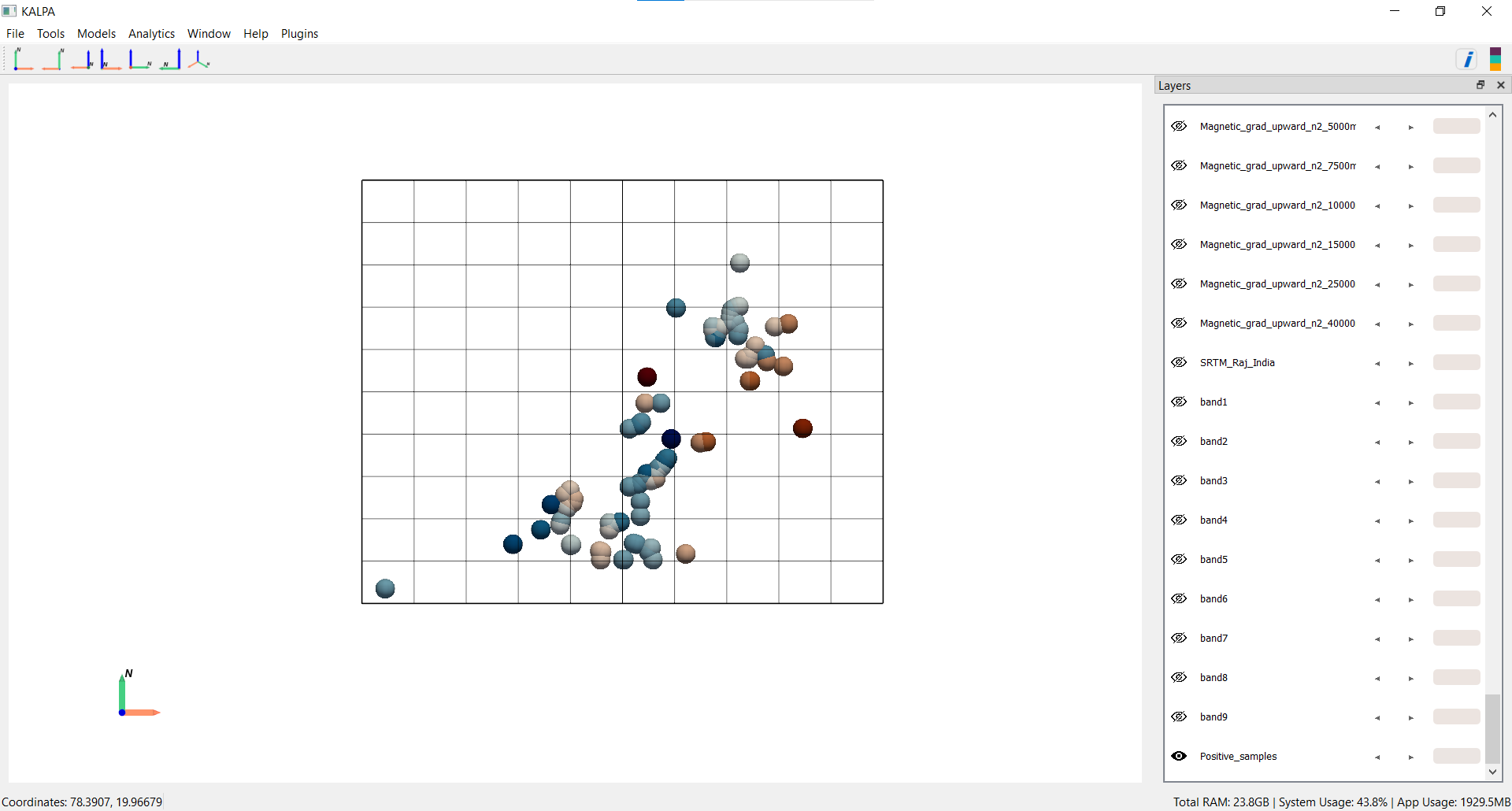
Step 1: Loading Data and Visualization

• Start Kalpa and create a new folder named MineralProspectivity to save the dataset, figures, etc.

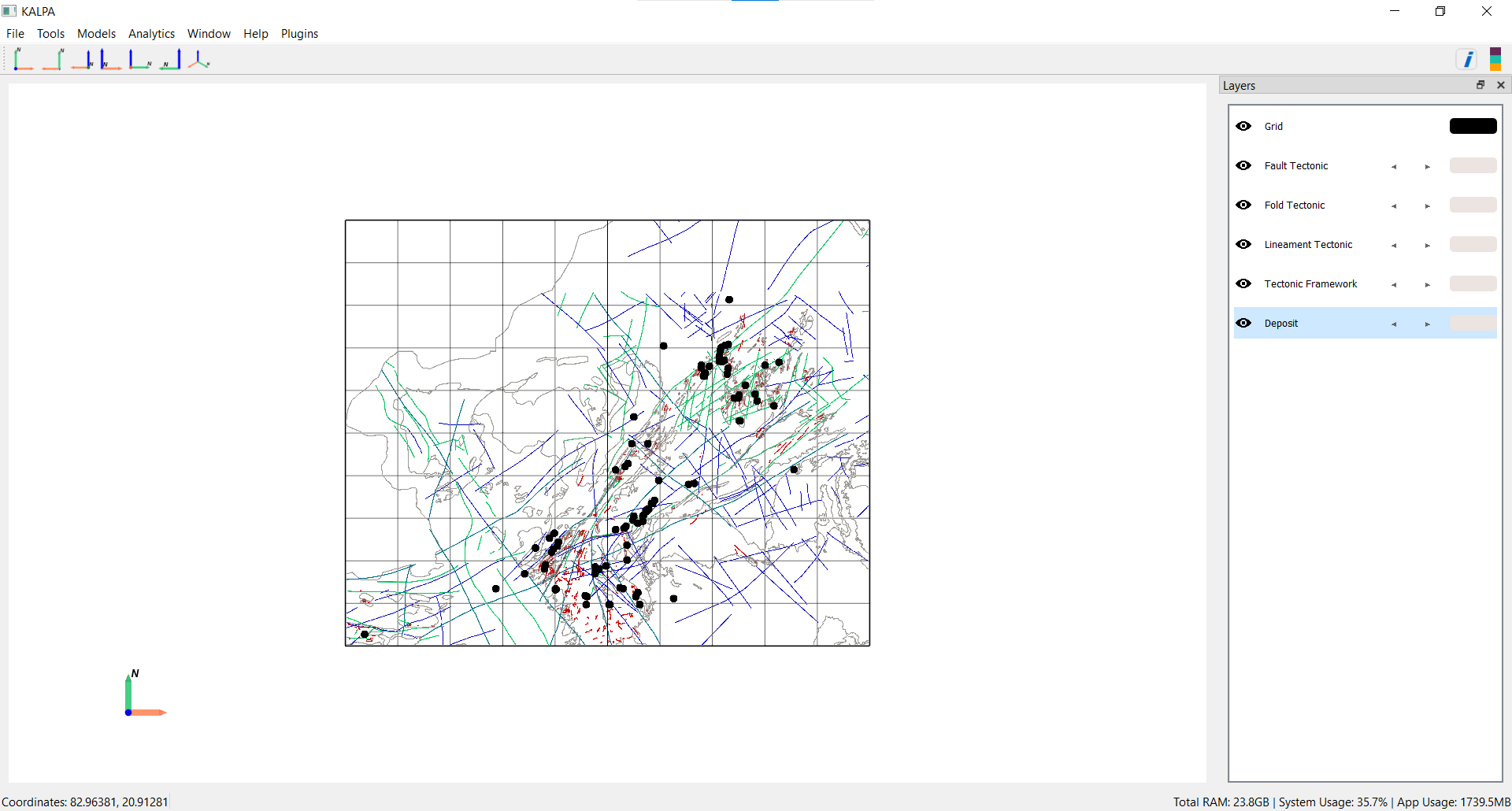
Import Vector Data:

• Navigate to File > Import > Vector Data.

• Load the following files:

  • ShapeFiles/Fault_Tectonic.shp

  • ShapeFiles/Fold_Tectonic.shp

  • ShapeFiles/Lineament_Tectonic.shp

  • ShapeFiles/Tectonic_Framework.shp

  • Deposits/Deposits.shp

• Adjust colormap, feature width, and range as needed.

  

Import Raster Data:

• Navigate to File > Import > Raster Data.

• Load the following files:

  • GeophysicalProcessed/Raster/BOUGUER_AN_Kriging.nc

  • GeophysicalProcessed/Raster/MAGNETIC_A_Kriging.nc

  • GeophysicalProcessed/Raster/Grad_Gravity/*

  • GeophysicalProcessed/Raster/Grad_Magnetic/*

  • GeophysicalProcessed/Raster/UC_Gravity/*

  • GeophysicalProcessed/Raster/UC_Magnetic/*

  • SatelliteData/SRTM/SRTM_Raj_India.nc

  • SatelliteData/LANDSAT/Band_1_LANDSAT.nc to Band_9_LANDSAT.nc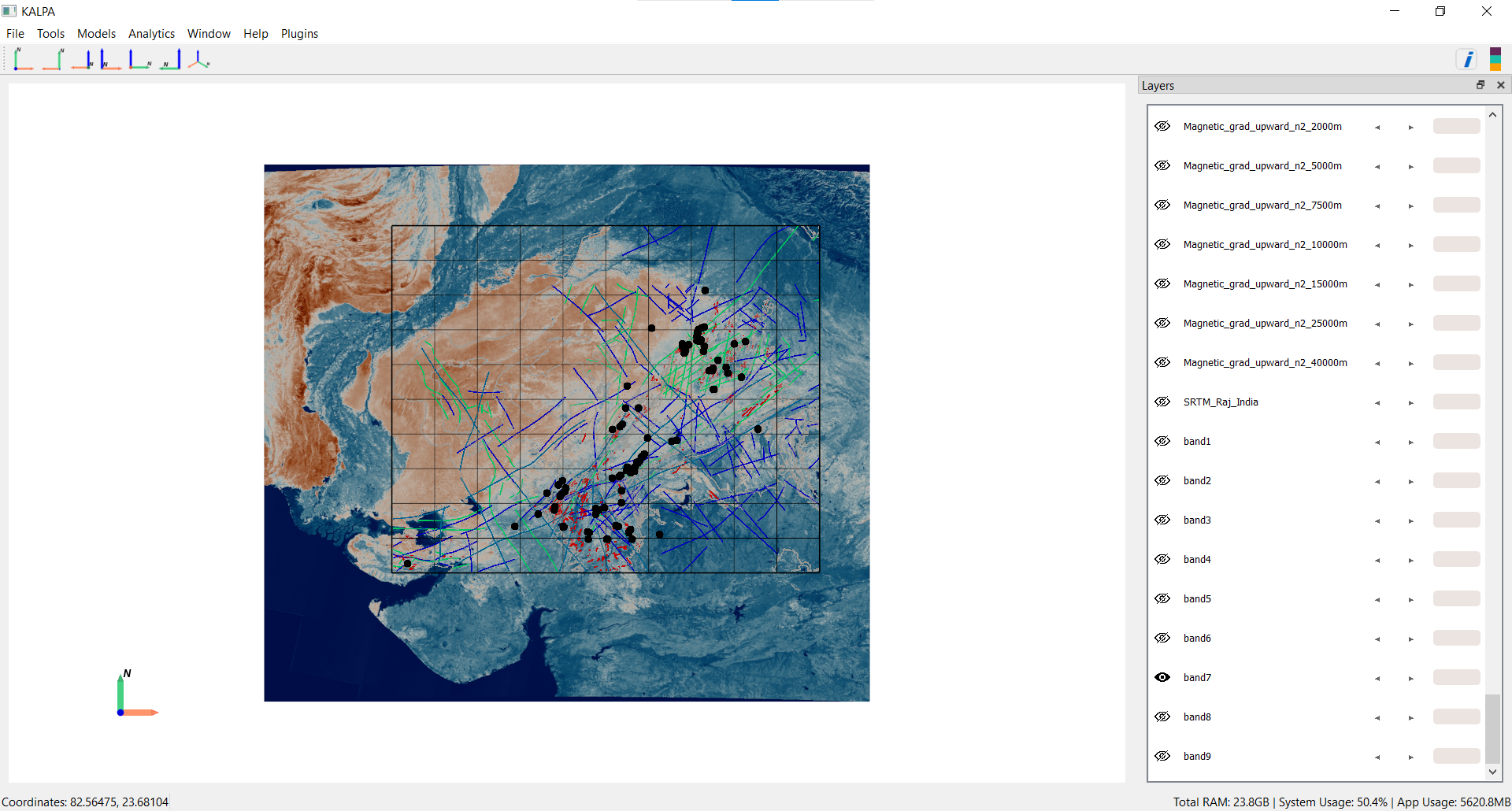

    

Step 2: Feature Generation

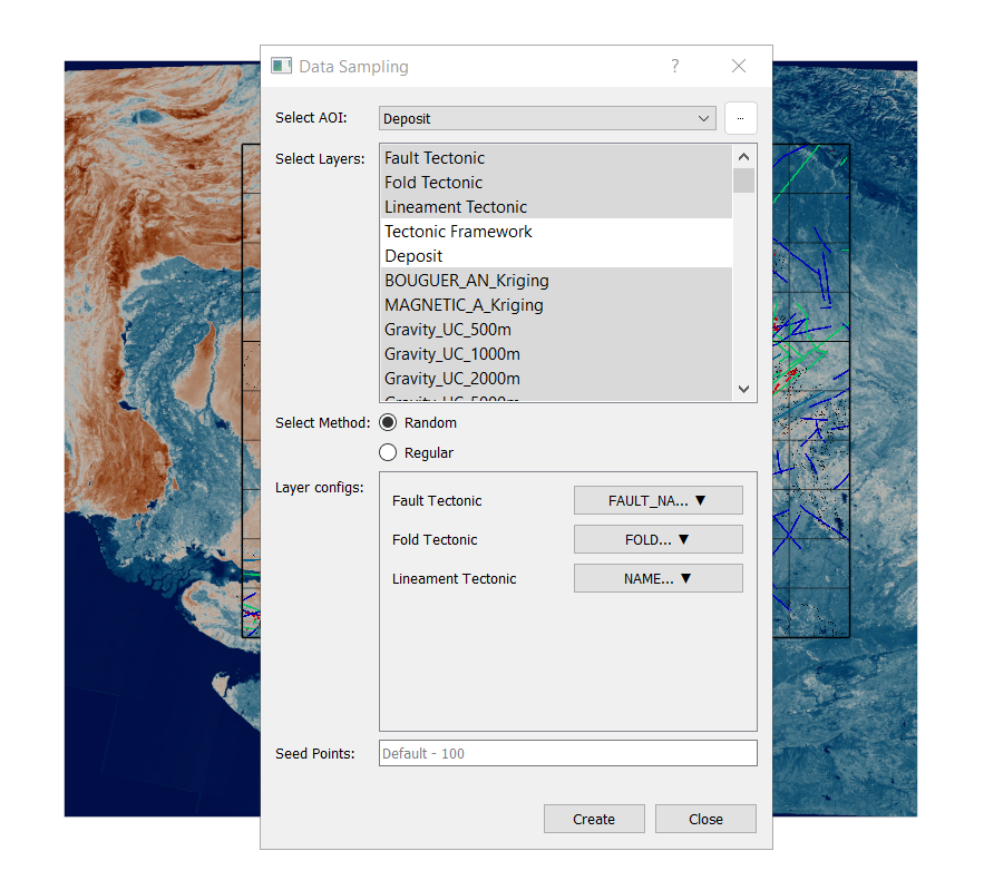
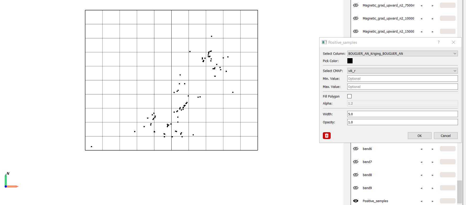
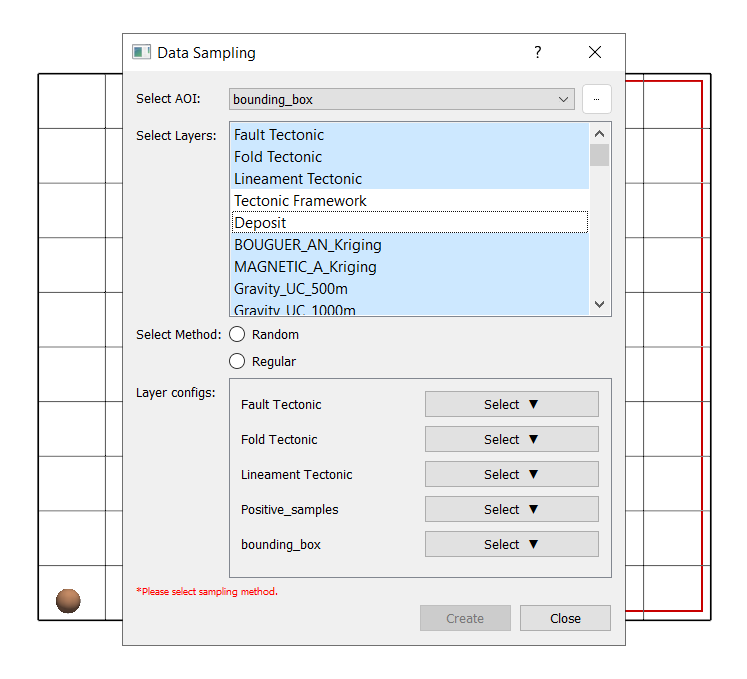
1. Generate Positive Labels from Known Deposits:

   • Navigate to Tools → Data Sampling.

   • AOI (Area of Interest): Deposit.

   • Select all layers except Tectonic Framework and Deposit.

   Layer Configuration:

   • Select the columns to be sampled for vectors having multiple columns:

     • Fault_Tectonic

     • Fold_Tectonic

     • Lineament_Tectonic

   • For rasters, select Band Value in case of multiple bands.

   • Sampling method: Random with default seed points as number of deposits are less than default value in this case.

   

   • Click Create → Save as: Positive_samples.gpkg.

   

   

2. Create Bounding Box:

   • Navigate to Tools → Vector → Bounding Box.

   • Select layer: BOUGUER_AN_Kriging

   

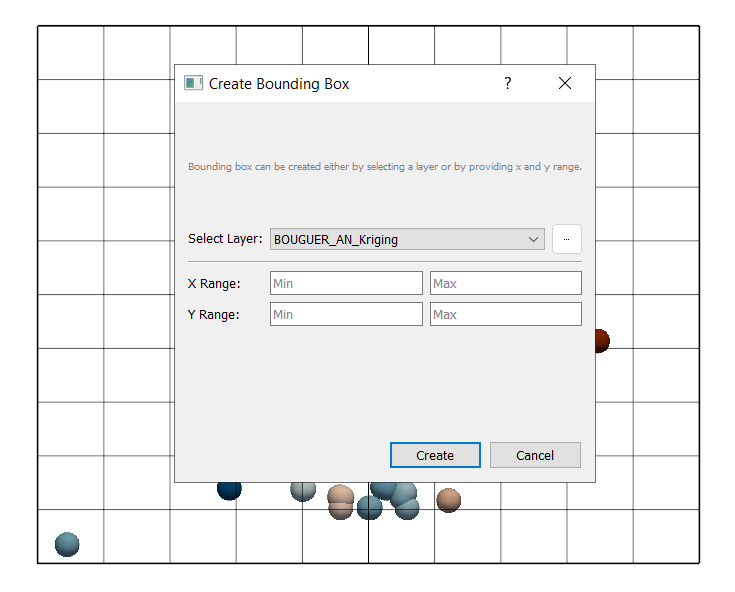
   • Click Create → Save as: bounding_box.gpkg.

   

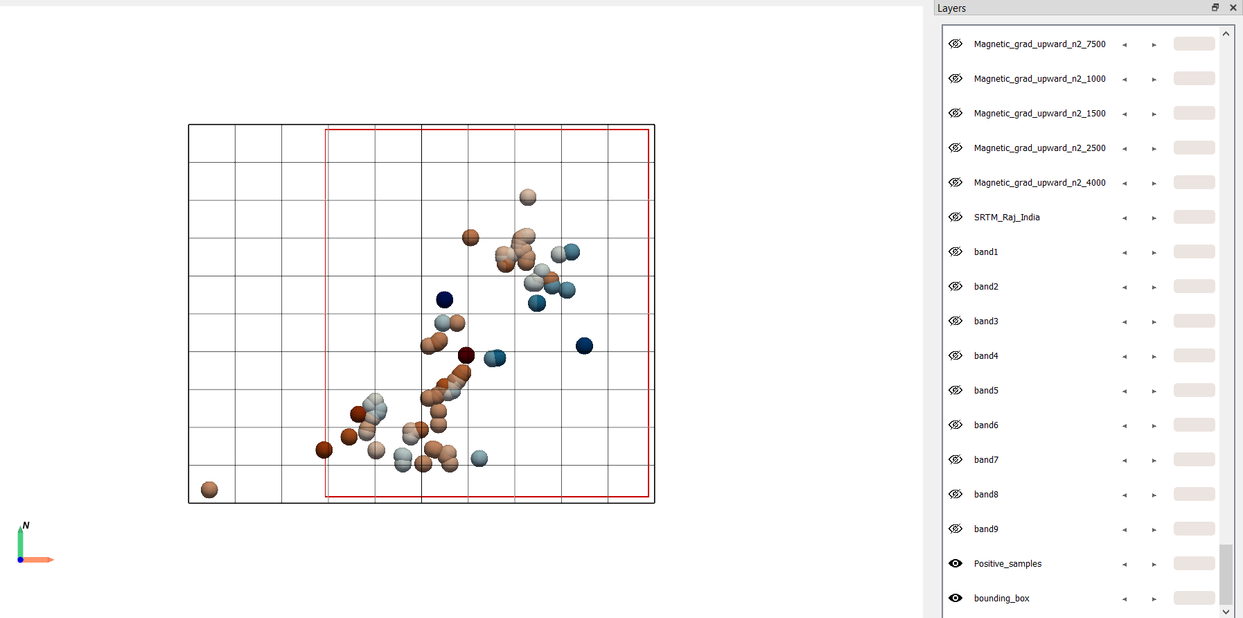
3. Generate Unlabelled Features:

   • AOI: bounding_box.

   • Select all layers except Tectonic Framework, Deposit, bounding_box, Positive_samples.

   • Method: Random, 3000 seed points.

   Layer Config:

   • Select the columns to be sampled for vectors having multiple columns:

     • Fault_Tectonic

     • Fold_Tectonic

     • Lineament_Tectonic

   

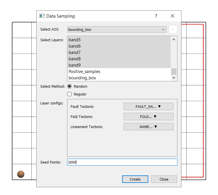
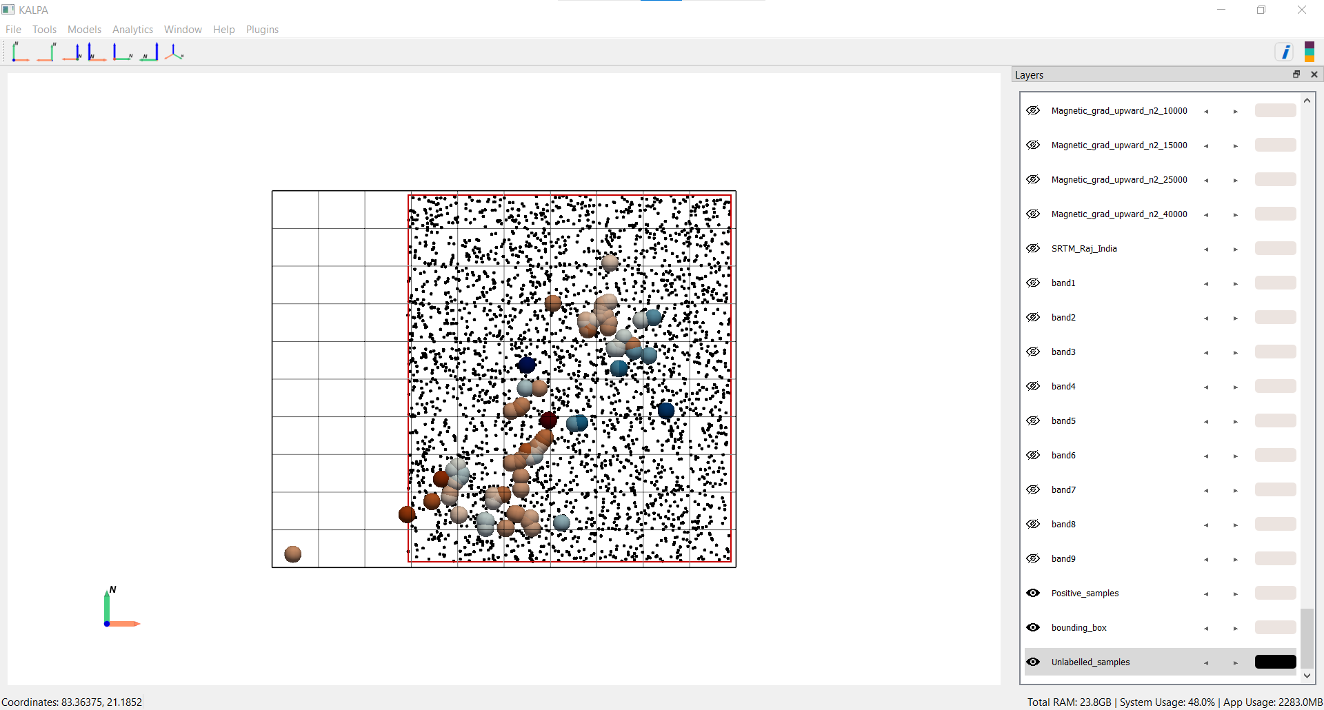
   • Click Create.

   

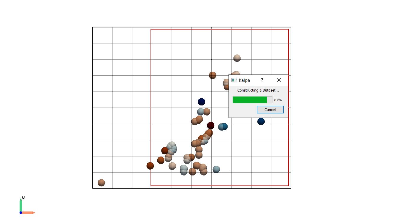
   • Save as: Unlabelled_samples.gpkg

   

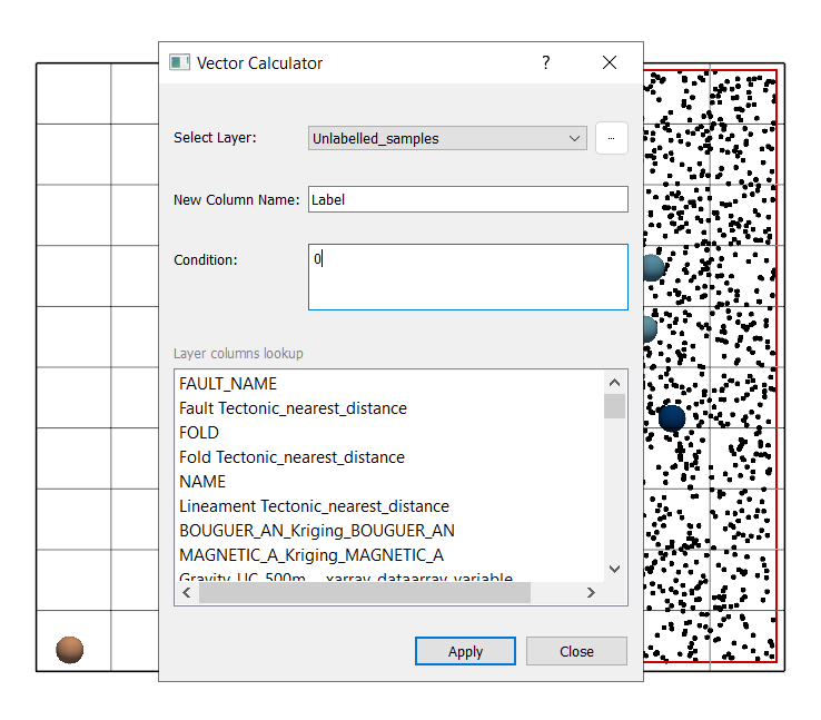
4. Generate Label Column:

   • Navigate to Tools → Vector → Calculator.

   • Layer: Positive_samples.

   • Condition: ‘1’ for positive samples.

   • Column name: Label.

   • Click Apply.

   

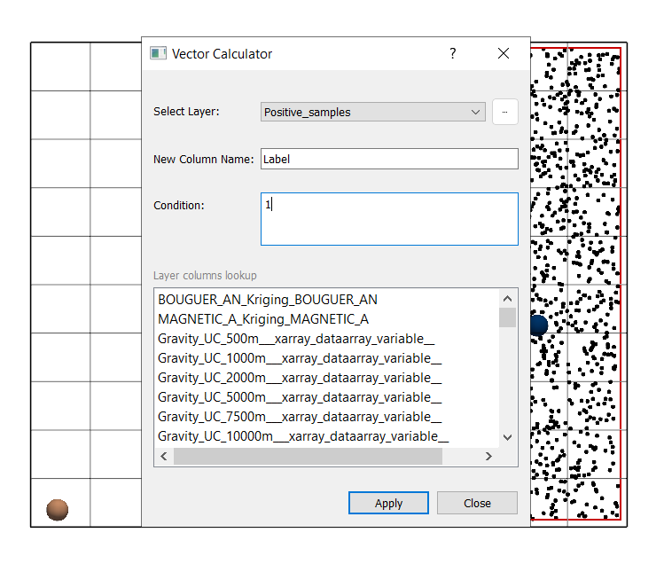
   • Save as: Positive_Label_calculated.gpkg

   • Repeat the same steps for Unlabelled_samples with condition ‘0’.

   • Save as: Negative_Label_calculated.gpkg

   

5. Merge Positive and Unlabelled Datasets:

   • Navigate to Tools → Vector → Merge Layers.

     

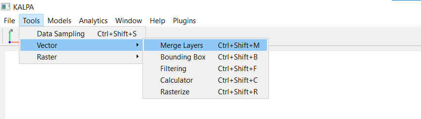
   • Layers: Positive_Label_calculated.gpkg and Negative_Label_calculated.gpkg.

   • Merge direction: Row Wise.

   • Click Merge.

     

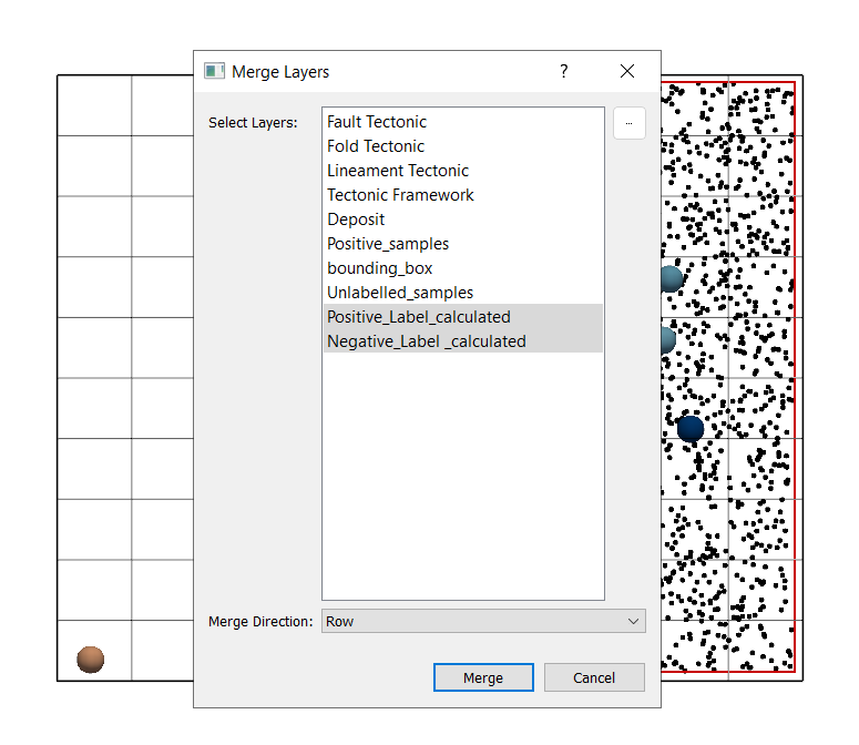
   • Save as: Training_Dataset.gpkg

     

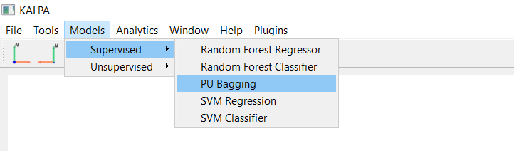
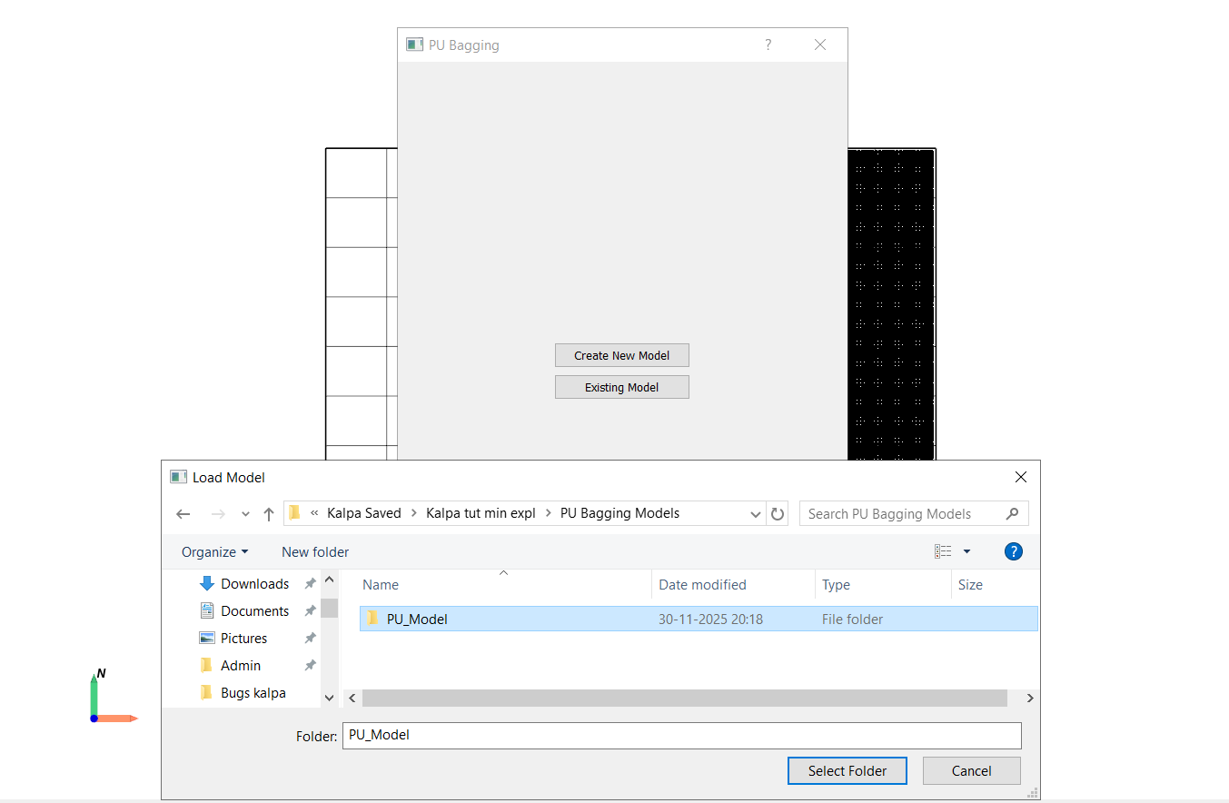
Step 3: Create PU Bagging Model

1. Navigate to Models → Supervised → PU Bagging.

   

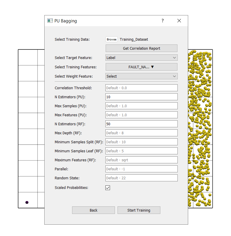
2. Select Create New Model.

3. Training data: Training_Dataset.gpkg.

4. (Optional) Generate correlation report to examine feature correlation.

5. Target feature: Label.

6. Select all other features as training features (except Label).

7. Tune other hyperparameters as needed.

8. Enable: scaled probabilities.

9. Click Start Training.

   

8. Save model as: PU_Model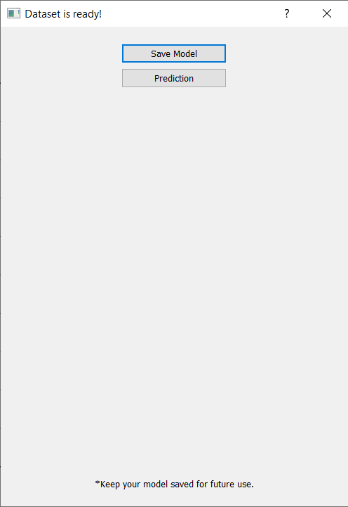

   

Step 4: Prediction and Visualization

1. Extracting Regular Grid for Prediction:

   • Navigate to Tools → Data Sampling.

   • AOI: bounding_box.

   • Select all layers except:

   • Tectonic Framework

   • Deposit

   • Positive_samples

   • Unlabelled_samples

   • bounding_box

   • Training_Dataset

   • Positive_Label_calculated

   • Negative_Label_calculated

   • Sampling method: Regular.

   • Set resolution to: 0.05 degrees. This may be of your choice.

     

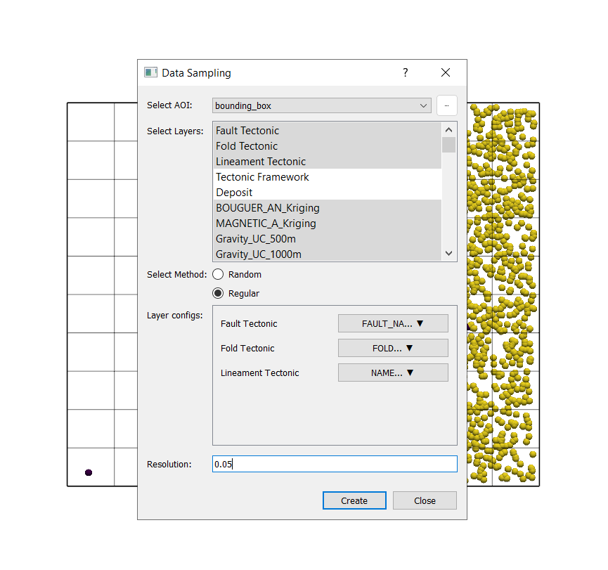
   • Click Create. Save as: Testing_Dataset.gpkg.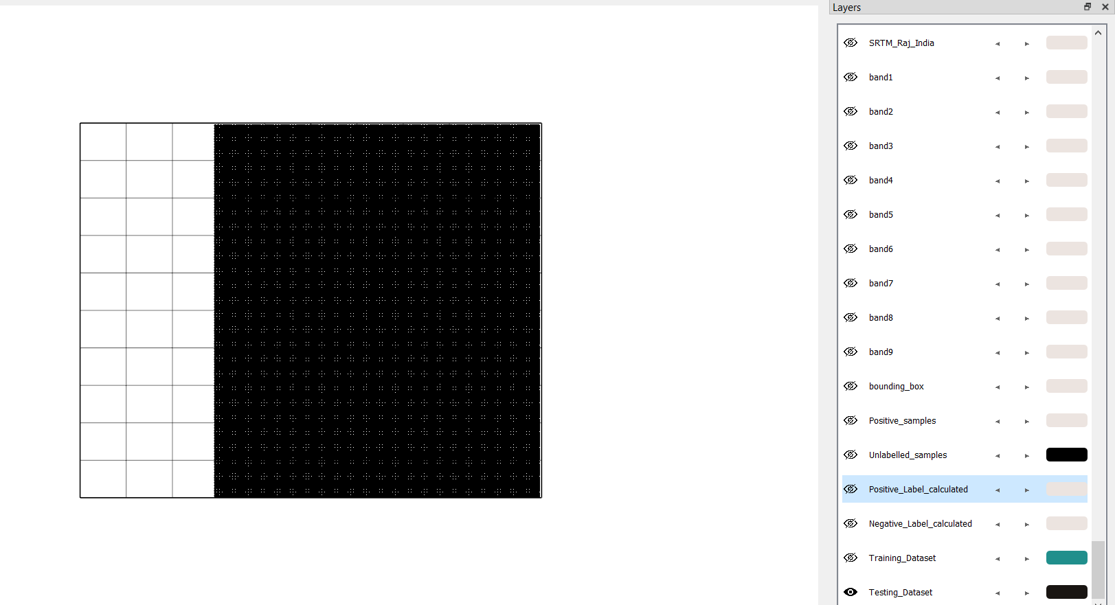

     

2. Prediction using Trained Model:

   • Navigate to Models → Supervised → PU Bagging.

     

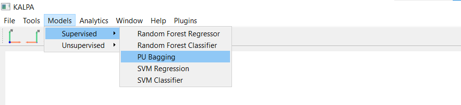
   • Select Existing Model.

   • Select PU_Model.

     

   • Choose: Testing_Dataset.gpkg as Data for Prediction.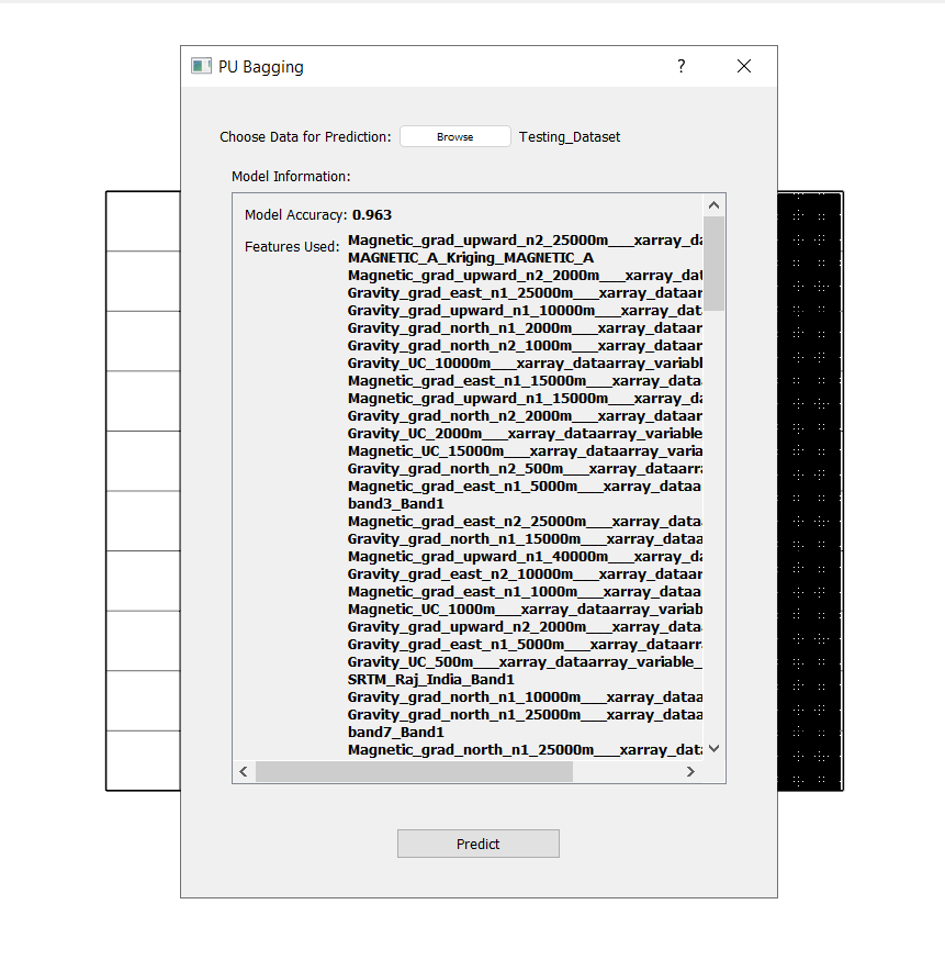

     

   • Click Predict

   • You now have your PU Bagging prediction.

     

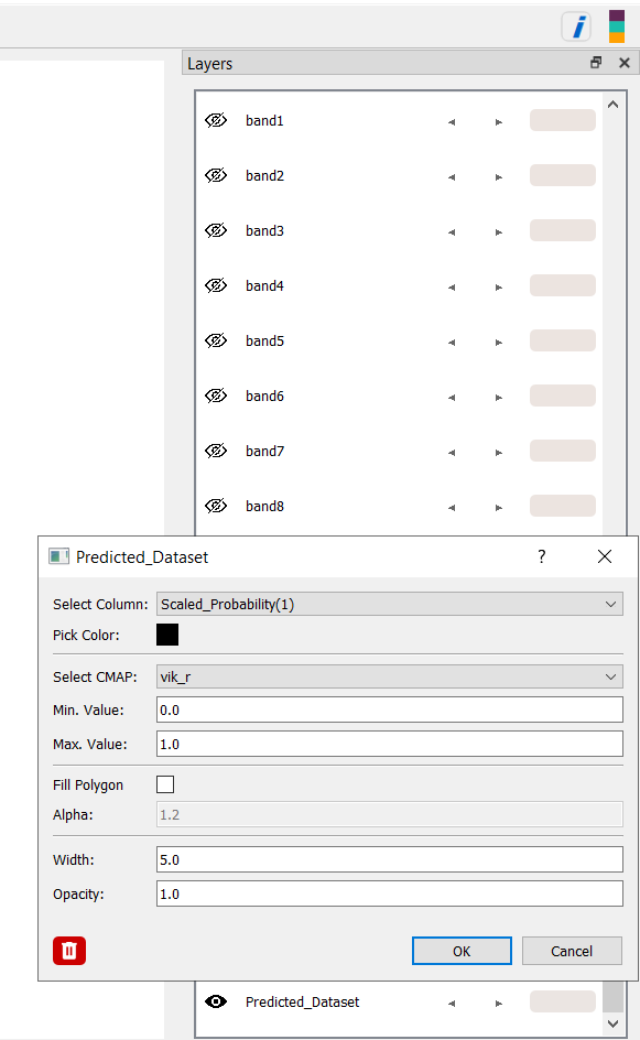
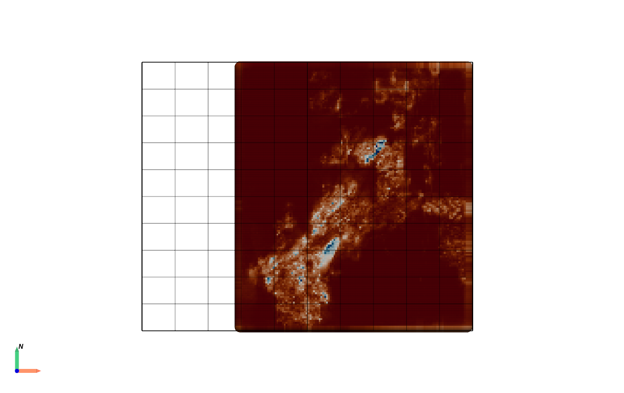
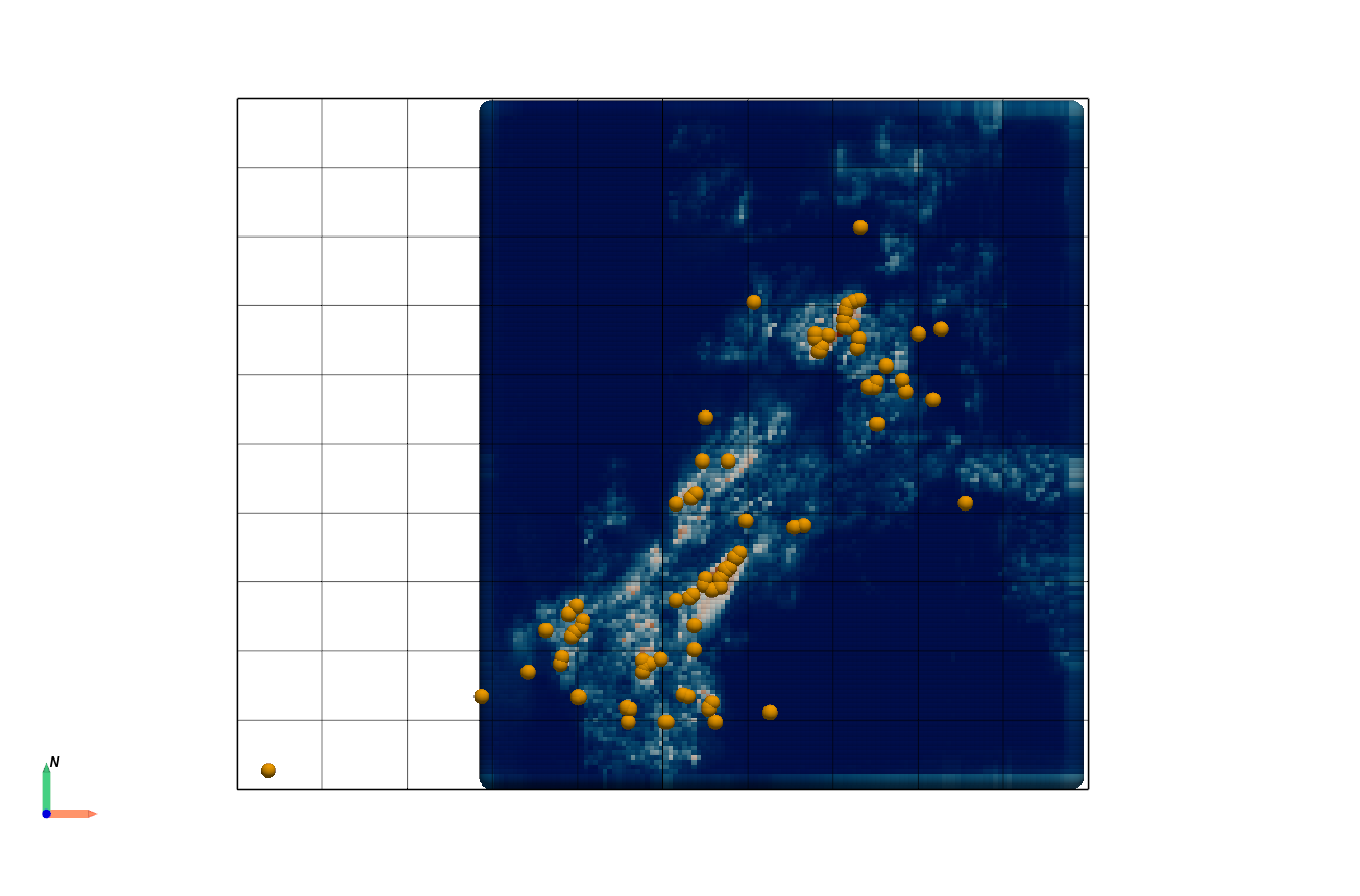
3. Visualizing Prospectivity Map:

   • Adjust colormap of your choice for better visualization and overlay the deposits layer to see how well the model has performed.