Geophysical Data Processing using Kalpa#
Kalpa offers a suite of tools for processing and analyzing geophysical data, enabling users to perform various operations such as filtering, transformation, and visualization. This section provides an overview of the key functionalities available in Kalpa for geophysical data processing.
Kriging Interpolation#
Kriging is a geostatistical interpolation method that provides optimal, unbiased predictions of spatially distributed variables. Kalpa supports kriging interpolation directly on vector data, allowing users to create continuous surfaces from discrete data points.
Function Overview#
Navigate to Plugins → Geophysics → Preprocessing → Kriging Interpolation.
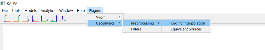
Select the input vector layer as File.
Choose the attribute column to interpolate.
Select the variogram model (e.g., Spherical, Exponential, Gaussian).
Set the output raster resolution.
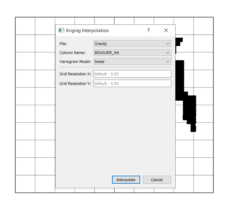
Click Interpolate to generate the interpolated raster layer.
Equivalent Sources#
Equivalent sources are used to model subsurface properties by representing complex geological structures with simpler, equivalent source distributions. Kalpa provides tool to create and analyze equivalent source models.
Function Overview#
Navigate to Plugins → Geophysics → Preprocessing → Equivalent Sources.
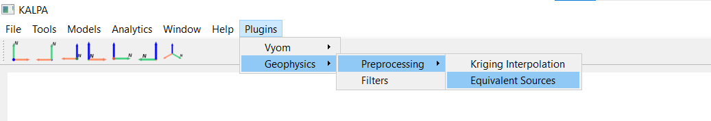
Select the input vector layer.
Choose the attribute column to model.
EQ Depth: Specify the depth of the equivalent source layer. This depth should be chosen based on the expected depth of the sources causing the observed anomalies.
Damping Factor: Set the regularization parameter to stabilize the inversion. A higher damping factor can reduce noise but may also smooth out real features.
Block Size: Define the size of the blocks used to divide the data area. Smaller blocks provide higher resolution but increase computational cost.
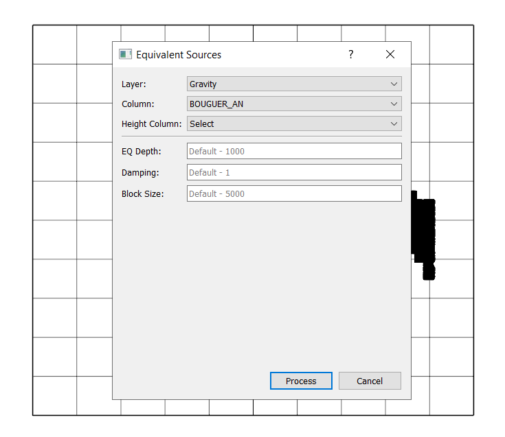
Click Process to create the equivalent source raster layer.
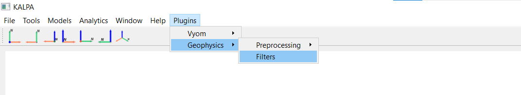
Geophysical Filtering operations#
Kalpa includes various geophysical filtering techniques to enhance and analyze geophysical data. These includes upward continuation, directional derivatives, Gaussian filters, etc.
Upward Continuation: Used to simulate the effect of measuring geophysical fields at a higher elevation, which helps in reducing near-surface noise.
Directional Derivatives: Calculate the rate of change of geophysical fields in specified directions, useful for identifying geological structures.
Derivative Northing: Calculates the derivative in the north-south direction.
Derivative Easting: Calculates the derivative in the east-west direction.
Derivative Upward: Calculates the derivative in the vertical direction.
Gaussian Filter: Applies a Gaussian smoothing filter to the geophysical data.
Gaussian Low Pass Filter: Smoothens the data by attenuating high-frequency components.
Gaussian High Pass Filter: Enhances high-frequency components by attenuating low-frequency components.
Total Gradient: Computes the total gradient magnitude of the geophysical field, which is useful for edge detection and highlighting geological boundaries.
Tilt Angle: Calculates the tilt angle of the geophysical field, aiding in the interpretation of subsurface structures.
Reduction to the Pole: Transforms magnetic data to simulate measurements as if taken at the magnetic pole, simplifying interpretation.
Function Overview#
Navigate to Plugins → Geophysics → Filters.
Select the raster layer to process.
Select the specific column within the raster layer (in case multiple columns are present).
Choose the desired filtering operation.
Configure any additional parameters required for the selected filter.
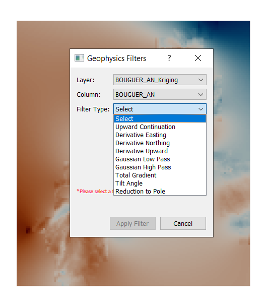
Click Apply Filter to execute the filtering operation and generate the output raster layer.